Simple Recurrent Neural Network (Simple RNN) @ FreelimbO | Friday, Aug 20, 2021 | 8 minutes read | Update at Friday, Aug 20, 2021

Layers: RNN, FC, and LogSoftmax.

By aggregating neural network layers, we are able to extract more abstract features beneficial to distinguish or classify examples. However, when it comes to temporal sequences with causality or nested embedding, MLPs and CNNs strand helplessly and typically require enormous numbers of neurons or kernels to capture seemly logical reasoning approaching the truth residing beneath the superficial appearance.

To illustrate the limitation of traditional neural networks, we are going to tackle a small task with two different methods, which are MLP and simple RNN. Suppose that we are simulating the addition of two 3-digit decimal numbers, the challenge for the models is to figure out the carry mechanism behind our customized dataset. We can easily calculate the addition because we have been taught to handle the carrys from lower digits to higher ones, and it must be done sequentially. Let’s get started to see if a shallow simple RNN can really emulated the addition.

Customized dataset for Addition

The dataset is generated randomly digit by digit with an uniform distribution of integers from 0 to 9. The first three examples of the dataset are shown in the table above for input features and labels, respectively. In each example, there are three pairs of integers denote for the units, tens, and hundreds digits from left to right. In other words, the first pair of 3-digit numbers is (438, 540), and the sum should be 978. This arrangement is similar with Little-Endian (LE) except for the radix is 10-base.

The shape of one example is $(\textbf{timeSeq}, \textbf{featureSize})$, which is an emulation of arithmetic of human minds and can be directly fed into an RNN. Nevertheless an MLP cannot handle the $\textbf{timeSeq}$-dimension, and therefore we reshape the all examples into of shape $(\textbf{timeSeq} \times \textbf{featureSize})$. The dataset has 1,000 examples, and we divide it into three parts (50%, 10%, 40%) for training, validation, and testing.

Models: MLP vs Simple RNN

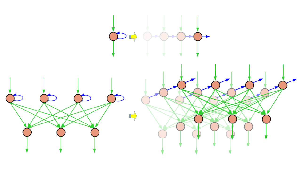
Besides an oridnary MLP, the recurrent model we use to tackle the 3-digit addition problem is an instance of Elman network. Elman network has only one recurrent layer composed with simple recurrent neurons. A simple recurrent neuron is an ordinary neuron just like the one of a fully-connected layer plus a directed self loop.

Since the capability of a network has strong relation with its number of learnable parameters, the upper limit of model sizes is set to 800 parameters. We design a 2-layer streamline multi-layer perceptron (MLP) of structure 20-30 and an simple RNN composed of one simple-RNN hidden layer with 21 neurons and one Linear Layer at the output layer with 10 neurons. The total numbers of parameters in the MLP and RNN are 770 and 745, respectively.

MLP Model Definition

 1
 2
 3
 4
 5
 6
 7
 8
 9
10
11
12
13
14
15
16
17

class MLPModel(nn.Module):
    def __init__(self, inputSize, outputSize, hiddenDim):
        super(MLPModel, self).__init__()
        self.hiddenDim = hiddenDim

        self.hFc = nn.Linear(inputSize, hiddenDim)
        self.fc = nn.Linear(hiddenDim, outputSize)
        self.sf = nn.LogSoftmax(dim=1)

    def forward(self, x):
        x = x.contiguous().view(x.shape[0], -1)
        self.hFcOut = self.hFc(x)
        self.hFcOut = self.hFcOut.contiguous().view(-1, self.hiddenDim)
        self.fcOut = self.fc(self.hFcOut)
        self.fcOut = self.fcOut.view(-1, 10)
        self.sfOut = self.sf(self.fcOut)
        return self.sfOut

(The display of python code is only correct in the dark mode. I will fix the light mode later.)

Simple RNN Model Defiintion

 1
 2
 3
 4
 5
 6
 7
 8
 9
10
11
12
13
14
15
16
17
18
19
20
21
22
23
24

class RNNModel(nn.Module):
    def __init__(self, inputSize, outputSize, hiddenDim, rnnLayers):
        super(RNNModel, self).__init__()
        self.hidenDim = hiddenDim
        self.rnnLayers = rnnLayers
        self.batchSize = 1

        self.rnn = nn.RNN(inputSize, hiddenDim, rnnLayers, batch_first=True)
        self.fc = nn.Linear(hiddenDim, outputSize)
        self.sf = nn.LogSoftmax(dim=1)

    def initRNNState(self):
        state = th.zeros(self.rnnLayers, self.batchSize, self.hiddenDim).to(device)
        return state
    
    def forward(self, x):
        self.batchSize = x.size(0)
        self.rnnState = self.initRNNState()
        self.rnnOut, _ = self.rnn(x, self.rnnState)
        self.rnnOut = self.rnnOut.contiguous().view(-1, self.hiddenDim)
        self.fcOut = self.fc(self.rnnOut)
        self.fcOut = self.fcOut.view(-1, 10)
        self.sfOut = self.sf(self.fcOut)
        return self.sfOut

The two models for the addition emulation task are defined as the two PyTorch modules shown above. We keep the two model definitions as similar as possible for readers to compare and focus on the difference among them. At the end of each model, we use log softmax layer to calculate the logit to accommodate the negative log likelihood loss function. Readers should have already understand the choices of logit layers and loss functions. It is noteworthy that the RNN model has an extra member function ${\bf initRNNState}$ to initialize the hidden state, which is critical because the hidden state takes parts in calculation of a recurrent neoron’s output and the next hidden state through the weight pointing back to each hidden recurrent neuron itself. The dimension of hidden state is of shape $(\textbf{batchSize}, \textbf{rnnLayers}, \textbf{hiddenSize})$, where $\textbf{rnnLayers}$ is the number of RNN layers, and $\textbf{hiddenSize}$ is the number of recurrent neurons. In the RNN model for the 3-digit addition task, we set the $\textbf{rnnLayer}$ to be 1.

Training Framework

 1
 2
 3
 4
 5
 6
 7
 8
 9
10
11
12
13
14
15
16
17
18
19
20
21
22
23
24
25
26
27
28
29
30
31
32
33
34
35
36
37
38
39

def predict(model, xCudaTensor):
    model.eval()
    prob = model(xCudaTensor)
    predict = th.max(prob, dim=1)[1]
    return predict

def testAcc(model, xCudaTensor, yCudaTensor):
    model.eval()
    pred = predict(model, xCudaTensor)
    pred = pred.reshape(yCudaTensor.shape).long()
    correct = yCudaTensor.eq(pred).all(dim=1).sum().item()
    model.train()
    return correct/pred.shape[0]

nPoints = 10
lossArray = th.zeros([nPoints])
accuracy = th.zeros_like(lossArray)
for epoch in range(1, nEpochs + 1):
    optimizer.zero_grad()
    indices = th.randperm(nTrBatches)

    for i in range(nTrBatches):
        x = trXCudaTensor[i*batchSize: (i+1)*batchSize]
        y = trYCudaTensor[i*batchSize: (i+1)*batchSize]

        prob = model(x)

        loss = criterion(prob, y.view(-1))

        loss.backward()
        optimizer.step()

    if epoch % (nEpochs//nPoints) == 0:
        j = epoch // (nEpochs//nPoints) -1
        lossArray[j] = loss.item()
        accuArray[j] = testAcc(model, vaXCudaTensor, vaYCudaTensor)

        print('Epoch: {:>5d}/{:>5d}......Loss: {:.4f}......Validation Accuracy: {:.2f}'
        .format(epoch, nEpochs, lossArray[j], accuArray[j]))

The three key parts of the network training framework are shown in the pythone code above. The ${\bf predict}$ function take an input CUDA FloatTensor of shape $(\textbf{batchSize}, \textbf{timeSeq}, \textbf{featureSize})$ and return a prediction of integer classes $\in \left [0, 9 \right ]$ of shape $(\textbf{batchSize}, \textbf{timeSeq})$. The {\bf testAcc} function wraps the prediction function with a post processing to calculate the validation/testing accuracy. The main body of the training includes a 2-layer nested loops. This outer loop iterates all epochs and validates the model periodically. The inner one feeds every mini-batch into the network model, performs the backprop for gradients, and updates the trainable parameters in the optimizer. This framework can be applied on the training procedures of the two models.

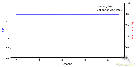
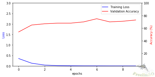
Figure 1. The learnign curves of MLP.	Figure 2. The learning curves of Simple RNN

We set the learning to be 0.0001 and use 20,000 epochs in total (We stop when anyone’s loss decreases below 0.001.) For the optimizer, we choose Adam because it often outperform SGD without incurring too much computational overhead. The learning curves of MLP and RNN are shown in Fig. 1 and 2. Obviously, the MLP with 770 trainable parameters fails to learn the 3-digit addition whilst the RNN with 745 trainable parameters succeeds at this task. The test accuracies of the two models are 0.25% and 76.25% for the MLP and RNN, respectively.

Results and Discussion

The failure of MLP and the success of RNN are actually two sides of one coin: the additional carry is a matter of temporal information. The MLP sees all input features of an example at once and can only extract spatial features. However, the RNN is equiped with self loops to bring back previous activations to join the current computation, which enables the model to understand temporal information. The table above lists some testing samples of the two trained models in the Little-Endian fashion. The first example is to add 334 with 135 and the correct sum should be 469. The MLP outputs an erroneous 246 and the RNN hit the correct answer. We can take a closer look at the following five samples and find out that the RNN still makes mistakes, but it has already figured out there must be a carry from the addition of the earlier pair of operands, and that carry needs to be added with the current addition. For the MLP model, we can hardly see anay correct or nearly correct predictions even on the unit digit (the digit related to the left most input pair), which has no existing carry to worry about.

The unfolding of a simple RNN neuron and Elman network.

Last but not least, the cover image shows the unfolding of an Elman network along the temporal axis. The blue arrows after being unfolded become the connections to a higher clone of the same layer (temporally later); thus the information of carries can find its path to affect the nearby digits.